Tutorial#
Introduction#
First you have to import the package.
In [1]: import evaltools as evt
In this package, the main class of objects is
Evaluator.
From an object of this kind you can compute all sort of statistics
and draw charts.
Classes Observations and
Simulations are precursors
of Evaluator. These two classes are
quite similar and the main way to instanciate them is by reading timeseries
files. What we call a timeseries file is a file containing two columns
separated by one or more space, the first column containing times (in
yyyymmddhh format) and the second column containing float values.
Examples of timeseries files can be found in “doc/sample_data”.
To begin working with Evaluator
objects you need a list of stations.
A example of a station listing is located in “doc/sample_data” and can be
read by
utils.read_listing.
In [2]: stations = evt.utils.read_listing("./sample_data/listing")

In [3]: stations
Out[3]:
        site area       lat       lon
code
AD0942A  bac  urb  42.50969   1.53914
AT0VOR1  bac  rur  46.67970  12.97190
AT10001  bac  sub  47.84000  16.52670
AT31401  bac  sub  48.08610  16.30220
AT31402  tra  sub  48.12500  16.33170
CH0002R  bac  rur  46.81310   6.94447
CH0005A  bac  sub  47.40290   8.61341
CH0005R  bac  rur  47.06740   8.46334
CH0010A  bac  urb  47.37760   8.53042
CZ0ALIB  bac  sub  50.00730  14.44590
CZ0HHKB  tra  urb  50.19540  15.84640
CZ0JKOS  bac  rur  49.57340  15.08030
CZ0PPLA  tra  urb  49.73240  13.40230
CZ0TOPR  ind  urb  49.85630  18.26970
We can now instanciate Observations
and Simulations objects from
“doc/sample_data” timseries files.
In [4]: from datetime import date

In [5]: start_date = date(2017, 6, 1)

In [6]: end_date = date(2017, 6, 6)

In [7]: observations = evt.Observations.from_time_series(
   ...:     generic_file_path="./sample_data/observations/{year}_co_{station}",
   ...:     correc_unit=1e9,
   ...:     species='co',
   ...:     start=start_date,
   ...:     end=end_date,
   ...:     stations = stations,
   ...:     forecast_horizon=2,
   ...: )
   ...:

In [8]: simulations = evt.Simulations.from_time_series(
   ...:     generic_file_path=(
   ...:         "./sample_data/ENSforecast/J{forecastDay}/{year}_co_{station}"
   ...:     ),
   ...:     stations_idx=stations.index,
   ...:     species='co',
   ...:     model='ENS',
   ...:     start=start_date,
   ...:     end=end_date,
   ...:     forecast_horizon=2,
   ...: )
   ...:
To understand the meaning of all the arguments, do not hesitate to refer to the API documentation.
Let’s create an Evaluator object and
start using its methods to compute statistics.
In [9]: eval_object = evt.Evaluator(observations, simulations)

In [10]: eval_object.temporal_scores(['RMSE', 'FracBias', 'PearsonR'])
Out[10]:
{'D0':                RMSE   FracBias  PearsonR
 code
 AD0942A         NaN        NaN       NaN
 AT0VOR1   66.870066  76.484397  0.456633
 AT10001   55.469560   2.077277  0.148668
 AT31401   32.292246  -4.318267  0.285162
 AT31402   28.410182  -1.741556  0.586555
 CH0002R   35.112389  24.917451  0.552076
 CH0005A   42.676788  12.441253  0.487120
 CH0005R   38.758369  24.589524  0.542966
 CH0010A   43.559315  -8.311611  0.448940
 CZ0ALIB  177.729834 -77.750712  0.452760
 CZ0HHKB   98.413269 -49.804323  0.303197
 CZ0JKOS   69.449904 -42.804008  0.366283
 CZ0PPLA  144.927767 -70.661566  0.262523
 CZ0TOPR  123.694578   8.622130 -0.022233,
 'D1':                RMSE   FracBias  PearsonR
 code
 AD0942A         NaN        NaN       NaN
 AT0VOR1   61.796662  72.098937  0.201367
 AT10001   52.191512 -14.062444  0.161187
 AT31401   32.975884  -6.221032  0.367900
 AT31402   30.017664  -2.887712  0.569830
 CH0002R   29.146724  21.548927  0.661740
 CH0005A   35.064446   6.494999  0.517632
 CH0005R   31.830369  19.650583  0.621802
 CH0010A   47.011353 -15.433575  0.430434
 CZ0ALIB  158.377078 -70.658442  0.670168
 CZ0HHKB   93.912730 -47.933881  0.434367
 CZ0JKOS   58.997009 -34.301921  0.678209
 CZ0PPLA  136.110242 -69.087018  0.496665
 CZ0TOPR  129.461101  13.036248  0.055859}
Plotting#
All plotting functions are gathered in
plotting
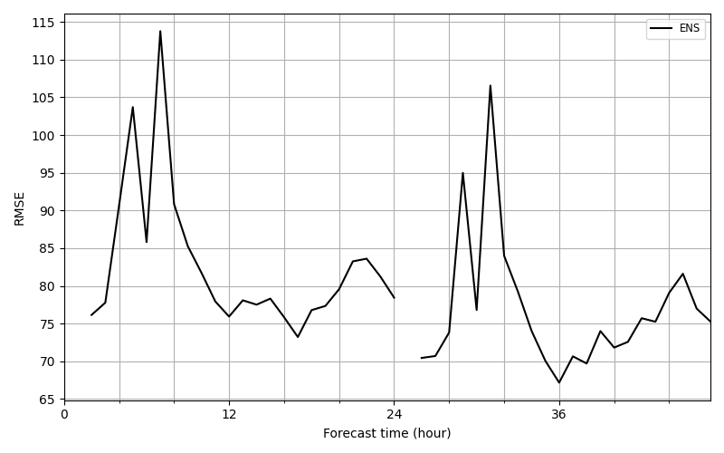
module. For instance, let’s draw mean RMSE over the 2 days forecast period with
plot_mean_time_scores
function.
In [11]: evt.plotting.plot_mean_time_scores(
   ....:     [eval_object],
   ....:     output_file="./source/charts/mean_RMSE_ENS",
   ....:     score='RMSE',
   ....: )
   ....:
Out[11]:
(<Figure size 800x500 with 1 Axes>,
 <Axes: xlabel='Forecast time (hour)', ylabel='RMSE'>)
And we get:
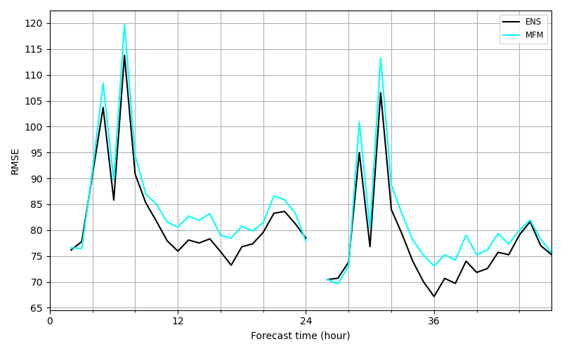
If we want more than one simulation drawn on the graph, we just have to
create other Evaluator objects and
pass them to the plotting function.
In [12]: simulations2 = evt.Simulations.from_time_series(
   ....:     generic_file_path=(
   ....:         "./sample_data/MFMforecast/J{forecastDay}/{year}_co_{station}"
   ....:     ),
   ....:     stations_idx=stations.index,
   ....:     species='co',
   ....:     model='MFM',
   ....:     start=start_date,
   ....:     end=end_date,
   ....:     forecast_horizon=2,
   ....: )
   ....:

In [13]: eval_object2 = evt.Evaluator(
   ....:     observations, simulations2, color='#00FFFF',
   ....: )
   ....:

In [14]: evt.plotting.plot_mean_time_scores(
   ....:     [eval_object, eval_object2],
   ....:     output_file="./source/charts/mean_RMSE_MFM",
   ....:     score='RMSE',
   ....: )
   ....:
Out[14]:
(<Figure size 800x500 with 1 Axes>,
 <Axes: xlabel='Forecast time (hour)', ylabel='RMSE'>)
And we get:
Different types of series#
Evaluator objects have a series type
attribute
In [15]: eval_object.series_type
Out[15]: 'hourly'
Here, the series type is "hourly". Indeed, when we construct an object
from timeseries file, it is the default value which means we work with
data measured at hourly time steps.
Some Evaluator methods will return an
object with seriesType attribute equal to "daily".
For instance,
In [16]: daily_max_object =  eval_object.daily_max()

In [17]: daily_max_object.series_type
Out[17]: 'daily'
We have thus created a new Evaluator
object which data is now composed of daily maximum values. Let’s compare
observation data held within eval_object and daily_max_object for a
given station.
In [18]: eval_object.obs_df['AT0VOR1']
Out[18]:
2017-06-01 00:00:00    52.42
2017-06-01 01:00:00    51.94
2017-06-01 02:00:00    52.91
2017-06-01 03:00:00    51.51
2017-06-01 04:00:00    50.15
                       ...
2017-06-07 19:00:00    63.87
2017-06-07 20:00:00    64.79
2017-06-07 21:00:00    63.82
2017-06-07 22:00:00    60.28
2017-06-07 23:00:00    61.20
Freq: h, Name: AT0VOR1, Length: 168, dtype: float64
In [19]: daily_max_object.obs_df['AT0VOR1']
Out[19]:
2017-06-01    62.95
2017-06-02    56.01
2017-06-03    81.38
2017-06-04    76.19
2017-06-05    59.85
2017-06-06    55.10
2017-06-07    64.79
Freq: 24h, Name: AT0VOR1, dtype: float64
Data with daily_max_object is given at daily time steps. Yet we can still
apply statical methods to this object to get scores per station for instance:
In [20]: daily_max_object.temporal_scores(['RMSE', 'FracBias', 'PearsonR'])
Out[20]:
{'D0':                RMSE   FracBias  PearsonR
 code
 AD0942A         NaN        NaN       NaN
 AT0VOR1   63.329672  65.026561  0.715997
 AT10001   63.759279 -23.786831 -0.041307
 AT31401   58.265557 -15.302091 -0.153068
 AT31402   46.254672 -14.800695  0.748693
 CH0002R   22.051733   0.446444  0.747533
 CH0005A   46.558323  15.454695  0.117165
 CH0005R   44.290206  26.646097  0.514922
 CH0010A   44.039217  -7.093002  0.368658
 CZ0ALIB  221.122365 -82.283008  0.340032
 CZ0HHKB  194.293000 -77.853086 -0.416637
 CZ0JKOS   82.474228 -46.437766  0.495443
 CZ0PPLA  257.489557 -90.305736 -0.277682
 CZ0TOPR  280.335540 -27.149906 -0.498600,
 'D1':                RMSE   FracBias  PearsonR
 code
 AD0942A         NaN        NaN       NaN
 AT0VOR1   58.092060  60.541266  0.387109
 AT10001   88.435543 -36.932643 -0.093816
 AT31401   51.828971 -18.108193  0.548205
 AT31402   43.623464 -14.001010  0.850362
 CH0002R   21.684452  -0.902961  0.833997
 CH0005A   46.927265   6.196613 -0.093322
 CH0005R   40.043196  24.650734  0.668365
 CH0010A   63.875332 -13.771354 -0.368416
 CZ0ALIB  198.456905 -77.289600  0.774305
 CZ0HHKB  185.439242 -74.547842  0.040638
 CZ0JKOS   70.772303 -39.570297  0.714519
 CZ0PPLA  175.483594 -77.518512  0.563888
 CZ0TOPR  279.958989 -27.023042 -0.171968}