Map plotting tools for gridded data

The quicklookmap module for plotting maps of 2D data from simulation outputs

Created on 24 Mai 2025

Authors:

radanovics

largely copied from epygram epy_cartoplot.py

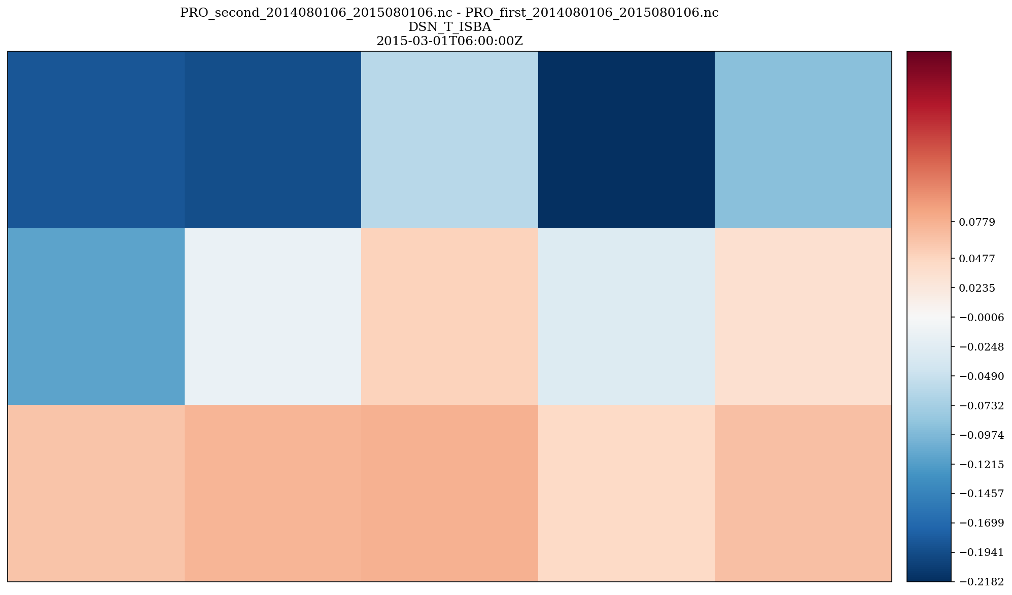
plots.maps.quicklookmap.difference_map(field, ref_field, title, plot_kwargs={})

Plot a difference map between two fields.

Parameters:

• field (epygram H2D field) – first scalar field

• ref_field (epygram H2D field) – reference field to substract.

• title (str) – plot title

• plot_kwargs – every other argument that can be passed to the cartoplot method of an epygram H2D field.

Returns:

dict with plot elements: ‘fig’, ‘ax’, potentially ‘colorbar’ etc.

Return type:

dict

plots.maps.quicklookmap.read_and_preprocess(resource, fid, date, operation=None, global_shift_center=None, zoom=None, additional_selection_options={})

Read field in resource, and preprocess if requested.

Parameters:

• resource (epygram.resource) – epygram resource to read data from

• fid (epygram field idenifier depending on the resource type. for example str for NetCDF files or a dict for grib files) – field identifier

• date (bronx.Date) – date (with time)

• operation (dict) – makes the requested operation (e.g. {‘operation’:’-‘,’operand’:273.15} or {‘operation’:’exp’}) on the field before plot. default=None

• global_shift_center – for global lon/lat grids, shift the center by the requested angle (in degrees). Enables a [0,360] grid to be shifted to a [-180,180] grid, for instance (with -180 argument).

• zoom (dict) – a dict(lonmin, lonmax, latmin, latmax) on which to build the plot.

Returns:

field

Return type:

epygram.field

Usage example (for getting total snow depth field of a 2D PRO file filename on a given date):

import epygram

from snowtools.plots.maps import quicklookmap

resource = epygram.formats.resource(filename, openmode='r')
field = quicklookmap.read_and_preprocess(resource, 'DSN_T_ISBA', '2021-12-01')

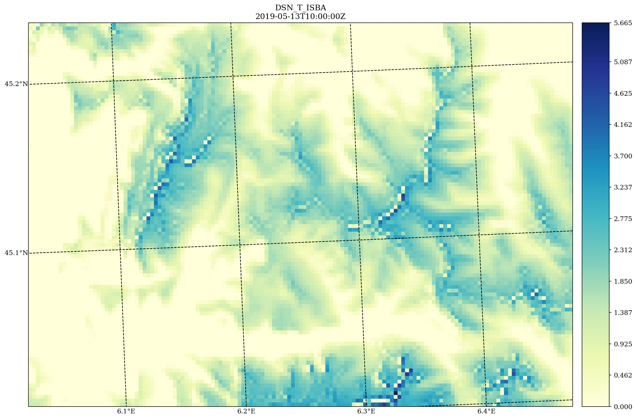
plots.maps.quicklookmap.scalar_map(field, title=None, plot_kwargs={})

Plot a map.

Parameters:

• field (epygram H2DField or H2DVectorField) – field to plot

• title (str) – plot title

• plot_kwargs – every other argument that can be passed to the cartoplot method of an epygram H2D field. Details can be found at: https://umr-cnrm.github.io/EPyGrAM-doc/library/H2DField.html#epygram.fields.H2DField.H2DField.cartoplot

Returns:

dict with plot elements: ‘fig’, ‘ax’, potentially ‘colorbar’ etc.

Return type:

dict

import maptplotlib.pyplot as plt

from snowtools.plots.maps import quicklookmap

quicklookmap.scalar_map(field)

plt.show()

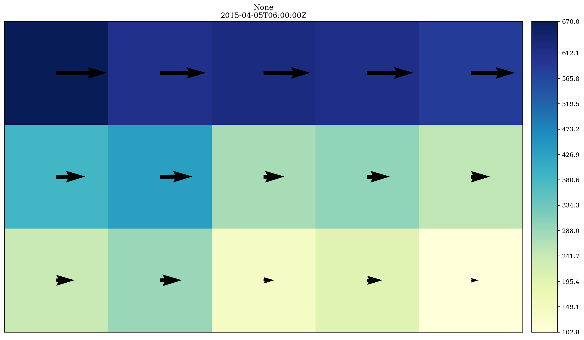
plots.maps.quicklookmap.wind_map(field, title, map_factor_correction=False, vectors_subsampling=50, wind_components_are_projected_on=None, vector_plot_method='quiver', quiverkey=None, plot_kwargs={})

Plot a map of a vector field.

Parameters:

• field (epygram vector field) – vector field to plot

• title (str) – plot title

• map_factor_correction (bool) – if True, applies a correction of magnitude to vector due to map factor.

• vectors_subsampling (int) – subsampling ratio of vectors plots. for example: 1 for a vector at every gridpoint, 10 for a vector every 10 grid points.

• wind_components_are_projected_on – inform the plot on which axes the vector components are projected on (‘grid’ or ‘lonlat’). If None (default), look for information in the field, or raise error.

• vector_plot_method – among (‘quiver’, ‘barbs’, ‘streamplot’) for vector plots. default is ‘quiver’.

• quiverkey – options to be passed to plotfield to activate a quiver key (cf. pyplot.quiverkey).

• plot_kwargs – every other argument that can be passed to the cartoplot method of an epygram H2D field. Details can be found at: https://umr-cnrm.github.io/EPyGrAM-doc/library/H2DField.html#epygram.fields.H2DField.H2DField.cartoplot

Returns:

dict with plot elements: ‘fig’, ‘ax’, potentially ‘colorbar’.

Return type:

dict

Helpers for pretty maps

A collection of functions to help pimping your cartopy maps !

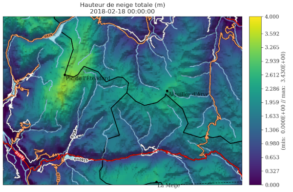
Use case example, I wanto to plot a total snow depth of a simulation with snowtools.plots.maps.quicklookmap and add a hillshade, some POIs, and a layer representing the hydrography.

import datetime

import matplotlib.pyplot as plt
import cartopy.crs as ccrs
import epygram

from snowtools.plots.maps import quicklookmap, map_helpers

projection = ccrs.epsg(9794)  # French Lambert projection
fig, ax = plt.subplots(1, 1, subplot_kw={'projection': projection}, figsize=(13, 6))

# Plot a scalar map of total snow depth
filename = '...'
date = datetime.datetime(2018, 2, 18)
resource = epygram.formats.resource(filename, openmode='r')
field = quicklookmap.read_and_preprocess(resource, 'DSN_T_ISBA', date)
quicklookmap.scalar_map(
    field,
    title=f"Hauteur de neige totale (m)",
    plot_kwargs={
        'fig': fig, 'ax': ax,
        'minmax': [0, 4],
        'colormap': 'viridis',
        'parallels': 'auto',
        'meridians': 'auto',
        'epygram_departments': True,
        'cartopy_features': []
    })

# Add points of interset
POI = [
    {'lat': 45.15449, 'lon': 6.143825, 'name': 'Pic de l'Étendard'},
    {'lat': 45.004942, 'lon': 6.309428, 'name': 'La Meije'},
    {'lat': 45.127064, 'lon': 6.336827, 'name': 'Aiguilles d'Arves'},
]

map_helpers.add_poi(ax, POIs=POI)

# Add a layer from IGN for rivers and hydrography
map_helpers.add_IGN_rivers(ax)

# Add an hillshade from IGN
map_helpers.add_IGN_hillshade(ax)

# Add road layer from IGN
map_helpers.add_IGN_feature(ax, layer='IGNF_TRANSPORTNETWORKS.ROADS')

plt.show()

plots.maps.map_helpers.add_IGN_feature(ax, layer, zorder=10, **kwargs)

Add a layer from the IGN map service on the cartopy map provided on axis ax.

For the list of layers available, see IGN documentation :

• https://data.geopf.fr/wms-r?SERVICE=WMS&VERSION=1.3.0&REQUEST=GetCapabilities

• https://cartes.gouv.fr/aide/fr/guides-utilisateur/utiliser-les-services-de-la-geoplateforme/tutoriels-api/qgis/

Parameters:

• ax – A maptpltlib Axis, with a projection defined

• layer (str) – Layer of the IGN index (str descriptor. e.g. : ELEVATION.ELEVATIONGRIDCOVERAGE.SHADOW)

• zorder (int) – Layer orderning (matplotlib index)

• kwargs – Arguments passed to matplotlib ax.imshow.

plots.maps.map_helpers.add_IGN_hillshade(ax)

Add an Hillshade for relief visualization (from IGN data).

plots.maps.map_helpers.add_IGN_rivers(ax)

Add a layer representing hydrography (from IGN data).

plots.maps.map_helpers.add_poi(ax, POIs, crs_ref='EPSG:4326', **kwargs)

Add point of interests on a map. POI is a list of points consisting of dictionnaries with key lat, lon (or x, y) and an optional ‘name’ to be plotted on the map.

Parameters:

• ax – A maptpltlib Axis, with a projection defined

• POIs (list of dict) – The list of the Point of interests

• crs_ref (str) – The CRS of the coordinates describing the POI (lat/lon or x, y). Defaults to lat/lon.

• kwarks – Arguments to be passes to ax.scatter (nb: marker, color and s are set resp. to o, k and 15 but can be overwritten).