Plotting modelled snow stratigraphy

The module of interest is plots/stratiprofile/profilPlot.

Created on 6 avr. 2017 Modified 7. apr. 2017 viallon

Authors:

• Pascal Hagenmuller

• Léo Viallon-Galinier

• Mathieu Fructus

plots.stratiprofile.profilPlot.dateProfil(axe, axe2, value, value_dz, value_grain=None, value_ram=None, xlimit=(None, None), ylimit=None, hauteur=None, color='b', cbar_show=False, legend=None, **kwargs)

Plot the vertical profile of the snowpack of one variable at a given date. If grain type and RAM resistance are given, these infos are added in the plot.

Parameters:

• axe (matplotlib axis) – figure axis

• axe2 (matplotlib axis) – figure axis (there are two axis on same plot: one for the variable, the other for snowgrain and RAM)

• value (numpy array) – variable to be plot

• value_dz (numpy array) – thickness value for all the layers considered

• value_grain (numpy array) – grain type for each layer

• value_ram (numpy array) – Résistance à l’enfoncement (traduction à trouver)

• xlimit (tuple) – give the x-limit for the variable (from limits_variable in proreader)

• ylimit (float) – give the upper y-limit for the variable (typically the snow depth)

• hauteur (float) – y-value for a black line in order to better see the interaction with seasonal profile

• color (boolean) – color name

• cbar_show – show the colorbar for grain type

• legend (datetime object or str) – legend (usually the date)

from snowtools.utils.prosimu import prosimu_auto
import matplotlib.pyplot as plt
from snowtools.plots.stratiprofile.profilPlot import dateProfil

point = 100
time = 100

with prosimu_auto('/rd/cenfic3/cenmod/home/viallonl/testbase/PRO/PRO_gdesRousses_2019-2020.nc') as ff:
    dz = ff.read('SNOWDZ', selectpoint=point, fill2zero=True)[time, :]
    var = ff.read('SNOWTEMP', selectpoint=point)[time, :]
    ram = ff.read('SNOWRAM', selectpoint=point)[time, :]
    grain = ff.read('SNOWTYPE', selectpoint=point)[time, :]
    time = ff.readtime()[time]

ax = plt.gca()
ax2 = ax.twiny()
dateProfil(ax, ax2, var, dz, value_grain=grain, value_ram=ram, legend=str(time))
plt.show()

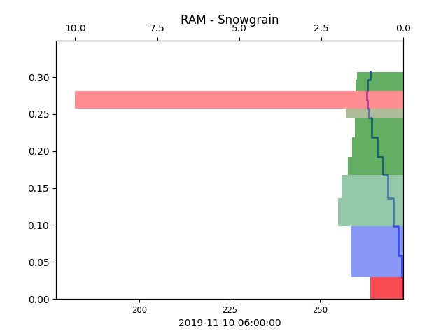
Example of plots that can be obtained with this function (example of the code snippet provided).

plots.stratiprofile.profilPlot.heightplot(ax, value, value_ep, time, legend=None, color='b', direction_cut='up', height_cut=10.0)

Plot the variable at a specific place in the snowpack. It is given with a height (in centimeter) and a direction. direction=’up’ means from ground to top of the snowpack direction=’down’ means from top of the snowpack to ground For example, if you want to plot 5 cm under the snowpack surface, you choose: height_cut=5 and direction_cut=’down’

Parameters:

• ax (matplotlib axis) – figure axis

• value (numpy array) – Value to be plot

• value_ep (numpy array) – thickness value for all the layers considered

• time (numpy array) – Time values

• color (str) – color name

• legend (str) – legend for the colorbar

• direction_cut (str) – legend for the colorbar

• height_cut (int) – legend for the colorbar

plots.stratiprofile.profilPlot.saison1d(ax, value, time, legend=None, color='b.', title=None, ylimit=None)

Plot the variable value across time for bulk variables (not variables per layer, e.g. total SWE, albedo, etc.).

Parameters:

• ax (matplotlib axis) – figure axis

• value (numpy array) – Value to be plot

• time (numpy array) – Time values

• legend (str) – legend for the colorbar

• color (str) – color name

• title (str) – title (date for member plots for example)

• ylimit (float) – give the upper y-limit for the variable (defaults to maximum snow depth)

from snowtools.utils.prosimu import prosimu_auto
import matplotlib.pyplot as plt
from snowtools.plots.stratiprofile.profilPlot import saison1d

point = 100

with prosimu_auto('/rd/cenfic3/cenmod/home/viallonl/testbase/PRO/PRO_gdesRousses_2019-2020.nc') as ff:
    var = ff.read('DSN_T_ISBA', selectpoint=point)
    time = ff.readtime()

ax = plt.gca()
saison1d(ax, var, time, title='Snow depth')
plt.show()

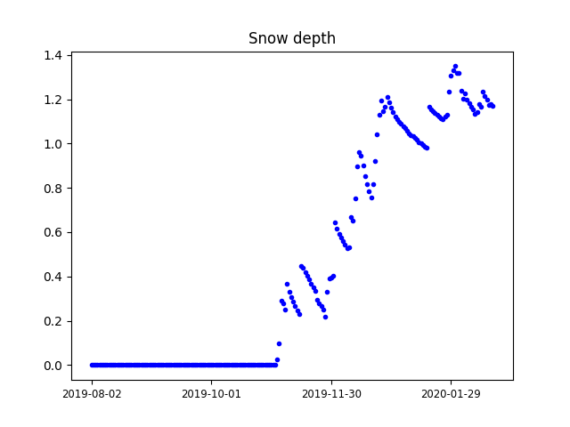
Example of plots that can be obtained with this function (example of the code snippet provided).

plots.stratiprofile.profilPlot.saisonProfil(ax, dz, value, time, colormap='viridis', value_min=None, value_max=None, legend=None, cbar_show=True, title=None, ylimit=None)

Plot a snow profile along time taking into account layer thicknesses for a realistic plot.

Parameters:

• ax (matplotlib axis) – figure axis

• dz (numpy array) – layer thicknesses

• value (numpy array) – Value to be plot (color of the layer). Should have the same dimension as dz

• time (numpy array) – Time values

• colormap (str or matplotlib colormap) – Colormap to use. Some custom colormaps are defined for specific variables: grains, echelle_log, echelle_log_sahara, ratio_cisaillement, tempK and lwc.

• legend (str) – legend for the colorbar

• value_min (float) – minimum value for colorbar

• value_max (float) – maximum value for colorbar

• cbar_show (bool) – Whether or not to plot the colorbar

• title (str) – title of the graph

• ylimit (float) – give the upper y-limit for the variable (defaults to the maximum snow depth across season)

Note that dz should not contain nan values. Layers that are not used sould be filled with a zero value for depth.

If you plan to add data, note that the x axis is not a time axis but an axis where the values are integers corresponding to the index of the date dimension (sue to limitations of the undelying matplotlib function).

Below is proposed a snippet of code that provide an example for such plot. Note that additional options may be necessary for some files (e.g. specification of tile).

from snowtools.utils.prosimu import prosimu_auto
import matplotlib.pyplot as plt
from snowtools.plots.stratiprofile.profilPlot import saisonProfil

point = 100

with prosimu_auto('/rd/cenfic3/cenmod/home/viallonl/testbase/PRO/PRO_gdesRousses_2019-2020.nc') as ff:
    dz = ff.read('SNOWDZ', selectpoint=point, fill2zero=True)
    var = ff.read('SNOWTYPE', selectpoint=point)
    time = ff.readtime()

ax = plt.gca()
saisonProfil(ax, dz, var, time, colormap='grains')
plt.show()

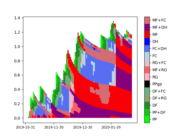
Example of plots that can be obtained with this function (example of the code snippet provided).